
Monitoring my daily activity
Published:
Ever since I bought my iPhone back in 2016, I carry it around in my pocket from pretty much the moment I wake up until I go to bed in the evening. All that time my phone has been recording my daily steps. After around 3 years, I thought it would be interesting to analyse my daily activity and see if I could learn some lessons. Spoiler alert: I did.
Import packages
import xml.etree.ElementTree
import numpy as np
import scipy as sp
from scipy.stats import boxcox
from scipy.special import inv_boxcox
import pandas as pd

import matplotlib.pyplot as plt
import matplotlib.dates as mdates
from matplotlib.pyplot import rcParams
import matplotlib.dates as mdates
%matplotlib inline
rcParams['font.sans-serif'] = "Arial"
rcParams['font.family'] = "sans-serif"

from datetime import date, datetime
Loading the data
Let’s start by importing the data. You can easily export your daily activity from the Health app on your iPhone. Just go to your profile, scroll all the way down and click on ‘Export All Health Data’. The following lines of code read in the ‘export.xml’ file and puts it into a more readable format.
xDoc = xml.etree.ElementTree.parse('export.xml')
items = list(xDoc.getroot()) # Convert the XML items to a list

# Loop through the XML items, appending samples with the requested identifier
tmp_data = []
item_type_identifier='HKQuantityTypeIdentifierStepCount' # Desired data type
for i,item in enumerate(items):
    if 'type' in item.attrib and item.attrib['type'] == item_type_identifier:
        # Attributes to extract from the current item
        tmp_data.append((item.attrib['creationDate'],
                         item.attrib['startDate'],
                         item.attrib['endDate'],
                         item.attrib['value']))

# Convert to data frame and numpy arrays
df = pd.DataFrame(tmp_data, columns = ['creationDate','startDate','endDate','steps'])
Getting the data in the right format
Next I want to clean up the DataFrame, so I can use it for later visualizations. I’ll create one DataFrame that has the data summarized per day and one per month.
# Convert colums
df.startDate = pd.to_datetime(df.startDate)
df.steps = pd.to_numeric(df.steps)

# Make date as index
df = df.set_index(df.startDate)

# Drop unnecessary columns
df = df.drop(columns=["creationDate","endDate","startDate"])

# Aggregate over days
df_day = df.resample('D').sum()

# Replace days with no recorded steps with the median number of steps
df_day['steps'] = df_day['steps'].replace(0,value=np.median(df_day['steps']))

# Average per month
df_month = df_day.resample('MS').mean()
Activity over the years
First, I would like to know how my activity has changed over the years. I will smooth the data slightly to make it a bit more visually pleasing. As a reference for all future analyses, the recommended number of steps per day is 10 000.
# Make data look a bit nicer by smoothing
df_smooth = df_month.rolling(window=4,center=True).mean()

# Settings
axfntsz = 20
axlabelfntsz = 24
lnwid = 4
transparency = .2
graphcol = [0.19, 0.23, 0.34]

# Create date locators
years = mdates.YearLocator()
months = mdates.MonthLocator()

## FIGURE

# Create actual figure
fig, ax = plt.subplots(figsize=(16, 6))
plt.fill_between(df_smooth.index,df_smooth.steps, color=graphcol, alpha=transparency)
plt.plot(df_smooth.index,df_smooth.steps, color=graphcol,linewidth=lnwid)

ax.xaxis.set_major_locator(years)
ax.xaxis.set_minor_locator(months)

plt.grid(which='both')
ax.set_axisbelow(True)

# Set labels
ax.xaxis.set_major_locator(years)
ax.tick_params(axis='x',labelsize=axlabelfntsz)
ax.tick_params(axis='y',labelsize=axfntsz)

plt.ylabel('Average steps',fontsize=axlabelfntsz)

ax.set_xlim(df_smooth.index[2],df_smooth.index[-2])
ax.set_ylim(0,10000)

plt.show()
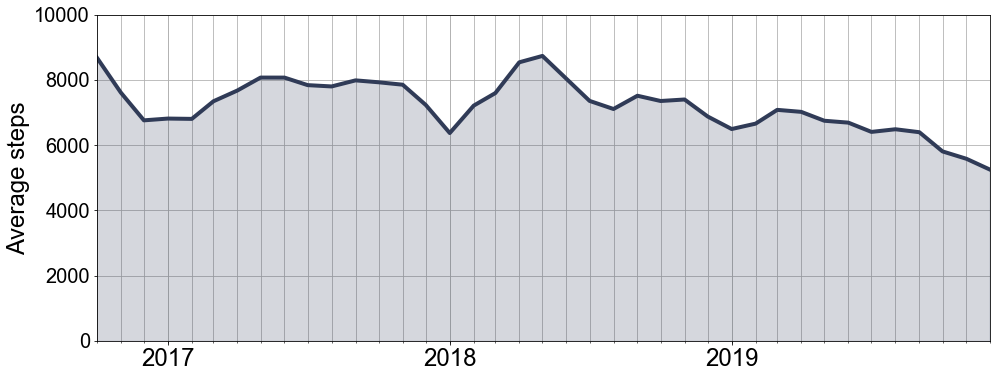
Alright, the first thing we can say for certain from this plot is that on average I have never met the mark of 10 000 steps a day. If we look a bit closer, it seems like in the earlier years I did get relatively close though. Over the years my activity seems to have dropped slightly. Let’s investigate!
Am I really getting more lazy?
To get a better handle on the trends in my data, I am going to fit a regression line to my daily step counts. If it is true that I am gradually moving less and less, we should see that the regression line slopes down.
(For visualization purposes, I have limited the y-axis to 10 000 steps, but obviously there were days where I did more than that.)
# Convert datetime to usuable format for polyfit
x = mdates.date2num(df_day.index)

# Fit regression line
coef = np.polyfit(x,df_day.steps,1)
poly1d_fn = np.poly1d(coef)

# Create actual figure
fig, ax = plt.subplots(figsize=(16, 6))
plt.plot(df_day.index,df_day.steps,'o', color='black',linewidth=lnwid,alpha=.5)
plt.plot(x,poly1d_fn(x),color='red',linewidth=3)

# Create grid
ax.xaxis.set_major_locator(years)
ax.xaxis.set_minor_locator(months)

plt.grid(which='both')
ax.set_axisbelow(True)

# Set labels
ax.xaxis.set_major_locator(years)
ax.tick_params(axis='x',labelsize=axlabelfntsz)
ax.tick_params(axis='y',labelsize=axfntsz)

plt.ylabel('Average steps',fontsize=axlabelfntsz)

ax.set_xlim(df_day.index[0],df_day.index[-1])
ax.set_ylim(0,10000)

plt.show()
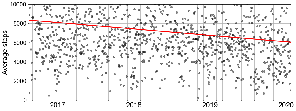
Auwch, that’s pretty clear. The fitted line slopes down quite a bit, indicating my activity levels have dropped. I could fit a second-order polynomial to the data to see whether there was a point where my activity started to fall more sharply rather than the constant decrease the regression line suggests. Instead, I want to take this one step further: given my current trend, what will my activity levels look like in 3 years time?
Predicting my future activity
To do so I will use the Prophet function from Facebook. The tool is highly convenient to use in modelling time series data and predicting future values. First I need create a DataFrame that is in the correct format. Contrary to my previous analyses, the datatime values should be a separate column, rather than the index. Once that’s done, we can enter the data into the function et voilà, out comes a model that can predict my future step count.
# First import the function
from fbprophet import Prophet
# Get data frame in right format
df = pd.DataFrame(tmp_data, columns = ['creationDate','startDate','endDate','steps'])

# Drop unnecessary columns
df = df.drop(columns=["creationDate","endDate"])

# Convert colums
df.startDate = pd.to_datetime(df.startDate)
df.steps = pd.to_numeric(df.steps)

# Aggregate over days
df_day = df.resample('D',on='startDate').sum()
df_day = df_day.reset_index()

# Rename columns
df_day = df_day.rename(columns={'startDate':'ds','steps':'y'})

# Replace missing values with median number of steps
df_day['y'] = df_day['y'].replace(0,value=np.median(df_day['y']))

# Clean up time series data with Box-Cox transform
df_day['y'], lam = boxcox(df_day['y'])
# Fit prophet model
m = Prophet(interval_width=0.95)
m.fit(df_day)
INFO:fbprophet.forecaster:Disabling daily seasonality. Run prophet with daily_seasonality=True to override this.


<fbprophet.forecaster.Prophet at 0x1c20bfb978>
# Add future days to model
future = m.make_future_dataframe(periods=36,freq='m')

# Predict future days
forecast = m.predict(future)

# Transform values back to interpretable values
forecast[['yhat','yhat_upper','yhat_lower']] = forecast[['yhat','yhat_upper','yhat_lower']].apply(lambda x: inv_boxcox(x, lam))
fig1 = m.plot(forecast)

fig1.set_size_inches(12, 6)
ax = plt.gca()

plt.ylabel('Steps',fontsize=axlabelfntsz)
plt.xlabel('Date',fontsize=axlabelfntsz)

ax.tick_params(labelsize=axfntsz)

plt.ylim(0, 20000)

plt.show()
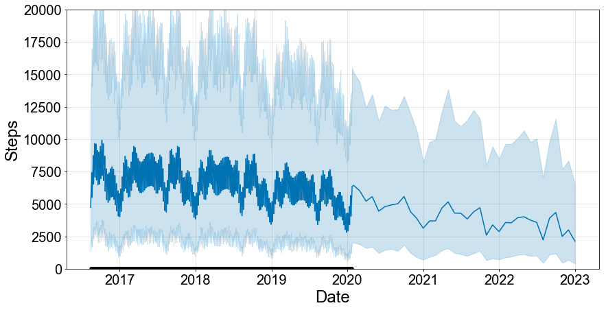
Things do not look better when I try to forecast my step count for the next 3 years. Based on the previous analysis, it was to be expected that my activity levels would further drop. At this rate I am down to a measly average of 2500 steps a day by 2023. However, silver lining, the 95%-confidence interval does leave some room for improvement. Given the uncertainty around these estimates, it is possible that my activity levels remains the same or even improves again.
For a final look at my general trends, Prophet allows you to separate the different components in your data. For example, you can expect to move more during the summer than during winter (more on that later). Similarly, you might sit behind a desk at work all week, but go on long hikes during the weekend. Plotting these different components can help to get a better grip on that data.
fig2 = m.plot_components(forecast,weekly_start=1)
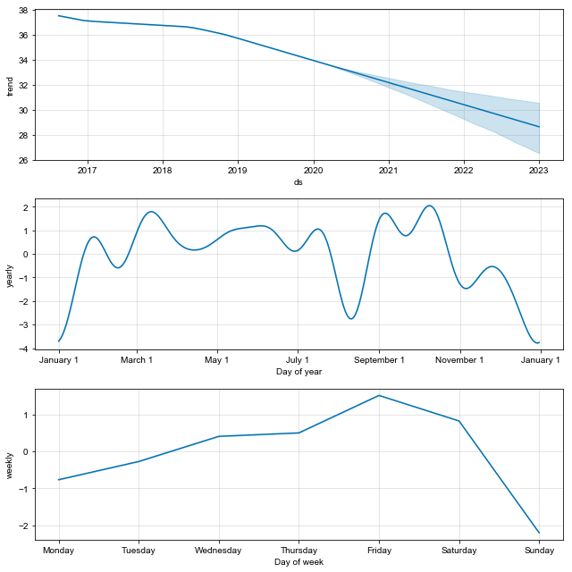
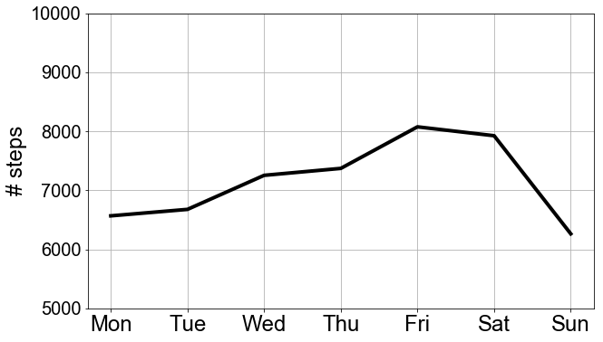
The top plot reiterates the same trend we’ve observed several times now (i.e. it’s all going down the drain). The middle plot tries to say something meaningful about my yearly activity. Because I have only accumulated a bit more than 3 years of data, these estimates should be slightly more noisy. Finally, the bottom plot shows my weekly activity. My activity peaks on the weekends, with a sharp drop on Sundays (clearly I like my lazy Sundays) and then gradually builds up to the weekend again.
Some more visualizations
I wanted to try out some more summary visualizations. We already saw the weekly and yearly activity thanks to Prophet, but I just wanted to plot them for myself too.
Weekly activity
# Aggregate over days
df_day = df.resample('D',on='startDate').sum()

# Add day indicator to data
df_day['weekday'] = df_day.index.dayofweek.astype('category')
df_day['weekday'] = df_day.weekday.cat.rename_categories(['Monday','Tuesday','Wednesday','Thursday','Friday','Saturday','Sunday'])

# Average over weekdays
plot_week = df_day.groupby('weekday')['steps'].mean()

# Plot weekly activity
fig, ax = plt.subplots(figsize=(10, 6))
plt.plot(plot_week.index.categories,plot_week.values,color='black',linewidth=lnwid)

plt.grid(which='both')
ax.set_axisbelow(True)

# Set labels
ax.set_xticklabels(['Mon','Tue','Wed','Thu','Fri','Sat','Sun'])
ax.tick_params(axis='x',labelsize=axlabelfntsz)
ax.tick_params(axis='y',labelsize=axfntsz)

plt.ylabel('# steps',fontsize=axlabelfntsz)

ax.set_ylim(5000,10000)

plt.show()
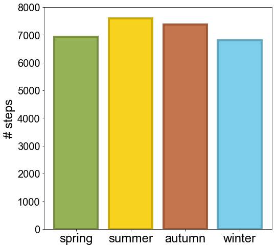
Seasonal activity
# Make function to indicate season
Y = 2000 # dummy leap year to allow input X-02-29 (leap day)
seasons = [('winter', (date(Y,  1,  1),  date(Y,  3, 20))),
           ('spring', (date(Y,  3, 21),  date(Y,  6, 20))),
           ('summer', (date(Y,  6, 21),  date(Y,  9, 22))),
           ('autumn', (date(Y,  9, 23),  date(Y, 12, 20))),
           ('winter', (date(Y, 12, 21),  date(Y, 12, 31)))]

def get_season(now):
    if isinstance(now, datetime):
        now = now.date()
    now = now.replace(year=Y)
    return next(season for season, (start, end) in seasons
                if start <= now <= end)

# Add indicator for season
df_day['season'] = df_day.index.to_series().apply(get_season)
df_day['season'] = df_day['season'].astype('category')

# Average over seasons
plot_season = df_day.groupby('season')['steps'].mean()
plot_season.index = plot_season.index.reorder_categories(['spring','summer','autumn','winter'])

# Figure

# Colours for spring/summer/autumn/winter
season_col = np.array([[139, 170, 67],[246, 205, 3],[190, 101, 57],[110, 201, 233]])/255

fig, ax = plt.subplots(figsize=(8, 8))

xval = plot_season.index.categories

plt.bar(plot_season.index.categories,plot_season.values, color=season_col,edgecolor=season_col*.8,alpha=.9,linewidth=lnwid)

# Set labels
ax.tick_params(axis='x',labelsize=axlabelfntsz)
ax.tick_params(axis='y',labelsize=axfntsz)

plt.ylabel('# steps',fontsize=axlabelfntsz)

ax.set_ylim(0,8000)

plt.show()
Conclusions
What is the take-home message here? Well, I clearly need to start moving around more. One thing the analysis does not take into account however is the time I spend playing squash or other sports. In other words, my phone only tracks my moderate activity levels. Nevertheless, the recommended number of steps is 10 000 independent of more physically intense activities.
It would have been interesting to do more ‘complex’ analyses, such as linking my activity to the daily temperature, precipitation etc. Unfortunately, I am too concerned about my privacy and did not have my location services turned on. Those analyses are going to have to wait another 3 years, when I’ve collected the data!