
It’s getting hot in here
Published:
For this project I wanted to learn a bit more about working with geographical data. We all (or at least the sensible ones among us) know the climate crisis is real, so I thought a nice starting point would be to track how the daily temperature in Belgium has evolved over the years, making the evolution of temperature over the decades a bit more tangible and personal. In my mind’s eye, the end product should be something that displays the temperature over the whole of Belgium and that you can manipulate to navigate between years.
The first challenge was to find an appropriate dataset. As a poor student, the requirements were that the data should be freely available and have a high enough resolution that the tiny country of Belgium has sufficient data points to plot. After some searching I found a dataset that met all criteria. The data I use is part of a larger dataset found here: Mistry, Malcolm Noshir (2019): A High-Resolution (0.25 degree) Historical Global Gridded Dataset of Climate Extreme Indices (1970-2016) using GLDAS data. PANGAEA, https://doi.org/10.1594/PANGAEA.898014, Supplement to: Mistry, MN (2019): A high resolution global gridded historical dataset of climate extreme indices. Data, 4(1), https://doi.org/10.3390/data4010041.
Loading packages
Some advice when working with all sorts of packages in Python and Anaconda/Miniconda. I lost a lot of time trying to figure out how to get my packages to work together, because of incompatibility problems. Personally I work with Miniconda3 and add more packages when needed. For the geographical data, I used GeoPandas, a variant of Pandas DataFrames that can work with geographical coordinates. But I ran into a lot of problems due to compatibility issues. I ended up with a fresh install of Miniconda3 and creating a separate environment for geographical data. I highly recommend you do the same! The new environment is also restricted to download from conda-forge, which helps with compatibility between packages. Do not forget to activate your environment before installing new packages or opening your project. Then you should be safe. You can find all instructions here.
import pandas as pd
import geopandas as gpd
import xarray as xr
import matplotlib.pyplot as plt

import numpy as np
from numpy.matlib import repmat

import scipy as sp
from scipy import interpolate

import ipywidgets as widgets
from ipywidgets import interact, interactive_output,fixed, IntSlider, Label, HBox
from IPython.display import display, Image

%matplotlib inline
The shape of you Belgium
Before diving into the data, I had to find an approriate shapefile. A shapefile contains a polygon with the coordinates for a country. I can then use this to visualize the borders of the country. But as you will see later I can also use it to determine the boundaries of my data. For these purposes I will create two GeoDataFrames: one that only contains the borders of Belgium for data limitation and another one that contains slightly more information for plotting.
# Load country file
project_folder = '/Users/fabriceluyckx/Documents/Projects/Temperature'
country_folder = project_folder + '/Belgium_shapefile'

# Load shapefile for plotting
gdf_plot = gpd.read_file(country_folder + '/gadm36_BEL_1.shp')
gdf_plot = gdf_plot.to_crs(epsg=4326)

# Load country outline for later use
gdf_be = gpd.read_file(country_folder + '/gadm36_BEL_0.shp')
gdf_be = gdf_be.to_crs(epsg=4326)
Getting our hands dirty
Alright, finally we can start to work with the data! Since the dataset contains data from across the world, there is a lot of redundant information here. I found a website that can determine a frame of coordinates around a country. I can then use those coordinates to limit the data I will be working with.
# Load data and convert to DataFrame
nc_f = project_folder + '/tmm_ANN_GLDAS_0p25_deg_hist_1970_2016.nc' # file name
ds = xr.open_dataset(nc_f)
df = ds.to_dataframe()

# Reshape to single index
df = df.reset_index(level=[0,1,2,3])

# Drop columns
df = df.drop(['bnds','time_bnds'],axis=1)

# Only keep rows that include Belgium (converting to gpd would take too long otherwise and redunant).
BE_frame = (2.39,6.41),(49.47,51.55)
df_BE = df[((df.lon >= BE_frame[0][0]) & (df.lon <= BE_frame[0][1])) & ((df.lat >= BE_frame[1][0]) & (df.lat <= BE_frame[1][1]))]
df_BE = df_BE.reset_index(drop=True)

# Create a column that only contains one year
df_BE['year'] = [i.year for i in df_BE.time]
df_BE = df_BE.drop(columns=['time'])
For the next step, I was a bit particular about the visualization. Even though the dataset is of ‘high resolution’ (it uses intervals of 0.25 degrees or around 27.75 km), for a country like Belgium, that is only 280 km wide, that means we only get around 10 data points next to each other. To make the plots look slightly better, I will interpolate the data to make things smoother. Note that I do the interpolation for the whole data set rather than when I start to subselect specific years. I chose to do it this way for speed. When you start scrolling between years and it still needs to interpolate the data, it will slow things down and make the experience less enjoyable.
# Interpolate data
# I found this method to deal much better with missing values than scipy's interp2d

nsteps = 150
xnew = np.linspace(np.min(df_BE.lon),np.max(df_BE.lon),nsteps)
ynew = np.linspace(np.min(df_BE.lat),np.max(df_BE.lat),nsteps)

df_interp = pd.DataFrame(columns=['year','lon','lat','tmm'])

for year in set(df_BE.year):

    df_year = df_BE[df_BE.year == year]

    # Get coordinates
    x = np.array(df_year.lon)
    y = np.array(df_year.lat)
    z = np.array(df_year.tmm)

    # Remove missing values
    x2 = list(x[np.isfinite(z)])
    y2 = list(y[np.isfinite(z)])
    z2 = list(z[np.isfinite(z)])

    znew = interpolate.griddata((x2, y2), z2, (xnew[None,:], ynew[:,None]), method='linear')

    # Put everything in a single DataFrame again
    tmp_df = pd.DataFrame(columns=['year','lon','lat','tmm'])
    tmp_df['year'] = repmat(year,nsteps**2,1).flatten()
    tmp_df['lon'] = repmat(xnew,nsteps,1).flatten()
    tmp_df['lat'] = repmat(ynew,nsteps,1).transpose().flatten()
    tmp_df['tmm'] = znew.flatten() # row-wise

    # Concatenate
    df_interp = pd.concat([df_interp,tmp_df])
It’s getting hot in here
Let’s start by plotting the temperature per year, to get a feel of the data. I fix the scale to have the minimum and maximum temperature between 1970 and 2016. This way we can observe the relative change in temperature. If I picked 0 degrees Celsius as the minimum of the scale, the differences would be barely noticeable. (Creating all subplots takes a while to run.)
years = list(set(df_BE.year))
nrows = int(np.ceil(np.sqrt(len(years))))
ncols = int(np.ceil(np.sqrt(len(years))))

# Determine absolute min and max
nlevels = 6
vmin, vmax = np.round([np.min(df_interp.tmm),np.max(df_interp.tmm)],2)

# Create figure
fig, axes = plt.subplots(nrows,ncols,figsize=(20,20))

for i in range(0,len(years)):

    ax = plt.subplot(nrows,ncols,i+1,frameon=False)

    # Select specific year
    df_year = df_interp[df_interp.year == years[i]]
    plotdat = df_year.pivot_table(index="lat",columns="lon",values="tmm")

    # Plot country outline
    gdf_plot.plot(color='none',edgecolor='black',ax=ax,zorder=2)

    # Overlay heatmap
    extent = [BE_frame[0][0] , BE_frame[0][1], BE_frame[1][0] , BE_frame[1][1]]
    plt.contourf(plotdat,cmap='YlOrRd',levels = nlevels-1,extent=extent,origin='lower',vmin=vmin,vmax=vmax,zorder=1)

    m = plt.cm.ScalarMappable(cmap='YlOrRd')
    m.set_array(plotdat)
    m.set_clim(vmin,vmax)

#    if i == 0:
#        cbar = plt.colorbar(m,
#                            ax=ax,
#                            shrink=.5,
#                            label='Average daily temperature',
#                            boundaries=np.linspace(vmin, vmax, nlevels).round(2))

    # Indicate the year
    ax.set_title("%d" % years[i],
                 {'fontsize' : 20,
                  'fontweight' : 'bold'})

    ax.axis('off')

# Remove redundant subplots
fig.delaxes(axes[nrows-1][ncols-2])
fig.delaxes(axes[nrows-1][ncols-1])

plt.tight_layout()
plt.show()

That’s quite a bit of data to gloss over. Eyeballing the different years it seems like the last decade has had more relatively hot years. But natural fluctuations make it hard to say anything decisive. Let’s summarize per decade, maybe that might make things a bit clearer.
# Define the decade's beginning and end
decades = np.array([[1970,1979],[1980,1989],[1990,1999],[2000,2009],[2010,2019]])
dec_names = ["70\'s","80\'s","90\'s","00\'s","10\'s"]

# Initialize dataframe
df_dec = pd.DataFrame(columns=['lon','lat','tmm','dec'])

for d in range(0,decades.shape[0]):

    df_tmp = df_interp[(df_interp.year >= decades[d,0]) & (df_interp.year <= decades[d,1])].groupby(['lat','lon'],as_index=False).mean()
    df_tmp['decade'] = repmat(dec_names[d],nsteps**2,1).flatten()

    # Concatenate
    df_dec = pd.concat([df_dec,df_tmp])
nrows = 1
ncols = len(dec_names)

# Determine absolute min and max
nlevels = 6
vmin, vmax = np.round([np.min(df_dec.tmm),np.max(df_dec.tmm)],2)

# Create figure
fig, axes = plt.subplots(nrows,ncols,figsize=(20,8))

for i in range(0,len(dec_names)):

    ax = plt.subplot(nrows,ncols,i+1,frameon=False)

    # Select specific decade
    df_plot = df_dec[df_dec.decade == dec_names[i]]
    plotdat = df_plot.pivot_table(index="lat",columns="lon",values="tmm")

    # Plot country outline
    gdf_plot.plot(color='none',edgecolor='black',ax=ax,zorder=2)

    # Overlay heatmap
    extent = [BE_frame[0][0] , BE_frame[0][1], BE_frame[1][0] , BE_frame[1][1]]
    plt.contourf(plotdat,cmap='YlOrRd',levels = nlevels-1,extent=extent,origin='lower',vmin=vmin,vmax=vmax,zorder=1)

    m = plt.cm.ScalarMappable(cmap='YlOrRd')
    m.set_array(plotdat)
    m.set_clim(vmin,vmax)

#    if i == 0:
#        cbar = plt.colorbar(m,
#                            ax=ax,
#                            shrink=.5,
#                            label='Average daily temperature',
#                            boundaries=np.linspace(vmin, vmax, nlevels).round(2))

    # Indicate the year
    ax.set_title("%s" % dec_names[i],
                 {'fontsize' : 20,
                  'fontweight' : 'bold'})

    ax.axis('off')

plt.tight_layout()
plt.show()

The same general trend comes out with average daily temperatures increasing over the decades. Note that the last decade was only halfway when this data set was made available, so conclusions here should be met with caution. Of course these data are not authoratative or conclusive, but they do suggest an alarming trend. At least my little exercise here is in line with what climate scientists have been saying for years: it’s getting hot in here!
An interactive map
Finally we can add some interactivity. First I will do something cool with GeoPandas. Since we have the shape of Belgium in a GeoDataFrame, I can use the sjoin function to only keep those data points that are within the borders of the country polygon.
# Only retain data within boundaries
gdf_interp = gpd.GeoDataFrame(df_interp, geometry=gpd.points_from_xy(df_interp.lon, df_interp.lat),crs='epsg:4326')
gdf_bound = gpd.sjoin(gdf_interp,gdf_be,op='within')
Because I want to add some interactive features, I will put the code within a function that takes the year as input. There are a lot of nice visualization tools that come with GeoPandas but after a lot of searching the simple matplotlib contourf function served my purposes best. Also note that I want to restrict the color scale so it is consistent over all years.
def plot_map(df_val,gdf_country,country_frame,Year=1970):

    # Select specific year
    df_year = df_val[df_val.year == Year]
    plotdat = df_year.pivot_table(index="lat",columns="lon",values="tmm")

    # Determine absolute min and max
    nlevels = 6
    vmin, vmax = np.round([np.min(df_val.tmm),np.max(df_val.tmm)],2)

    # Create figure
    fig, ax = plt.subplots(figsize=(15, 10))

    # Plot country outline
    gdf_country.plot(color='none',edgecolor='black',ax=ax,zorder=2)

    # Overlay heatmap
    extent = [country_frame[0][0] , country_frame[0][1], country_frame[1][0] , country_frame[1][1]]
    plt.contourf(plotdat,cmap='YlOrRd',levels = nlevels-1,extent=extent,origin='lower',vmin=vmin,vmax=vmax,zorder=1)

    m = plt.cm.ScalarMappable(cmap='YlOrRd')
    m.set_array(plotdat)
    m.set_clim(vmin,vmax)

    cbar = plt.colorbar(m,ax=ax,shrink=.5,label='Average daily temperature',boundaries=np.linspace(vmin, vmax, nlevels).round(2))

    ax.axis('off')

    plt.show()
Jupyter notebooks come with some simple interactive tools. You will need to follow a few steps to make them work within your notebook. Make sure to have the correct environment activated! In this case I just need a slider that can vary the year.
Year = widgets.IntSlider(min=1970,
                         max=2016,
                         step=1,
                         value=1970)

ui = widgets.HBox([Label('Year'), Year])

out = widgets.interactive_output(plot_map,{'df_val':fixed(gdf_bound),
                                           'gdf_country':fixed(gdf_plot),
                                           'country_frame':fixed(BE_frame),
                                           'Year':Year})
# the fixed argument makes sure I don't create an interactive tool for that specific input

display(ui, out)
HBox(children=(Label(value='Year'), IntSlider(value=1970, max=2016, min=1970)))


Output()
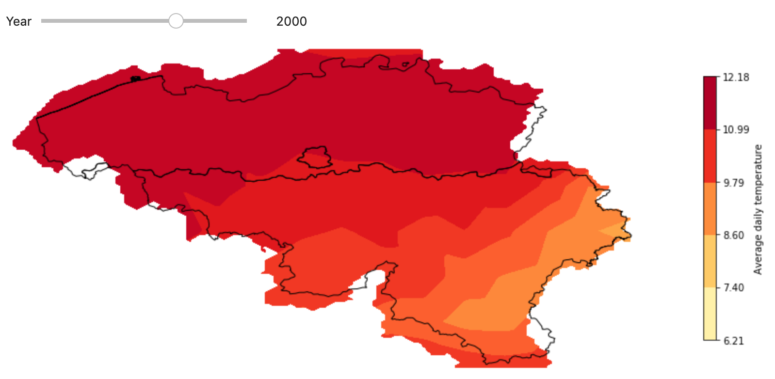
Annoyingly the interactive plot will not show up in Markdown. I will include a screenshot of the result below to give you an idea.
Image(filename='Ipywidget_screenshot.png')
For some reason the borders do not perfectly align between the temperature data and the country. When I have more time, I would like to figure out where exactly it went wrong. But for now, this will have to do!